How a Camera Interprets a 3D Point

Visual odometry (VO) estimates how a camera moves by comparing the images it records. Every VO method, whether it matches features, aligns pixel intensities directly, or uses a learned network, depends on a model of how a 3D point in front of the camera ends up at a particular pixel. That model is the pinhole camera model, and it is the subject of this first part of the series.

This post covers:

the pinhole model and the camera coordinate frame,
the projection equations and the intrinsic matrix \(K\),
a worked example, checked in NumPy and OpenCV,
going from a pixel back to a 3D ray.

1. The pinhole camera model

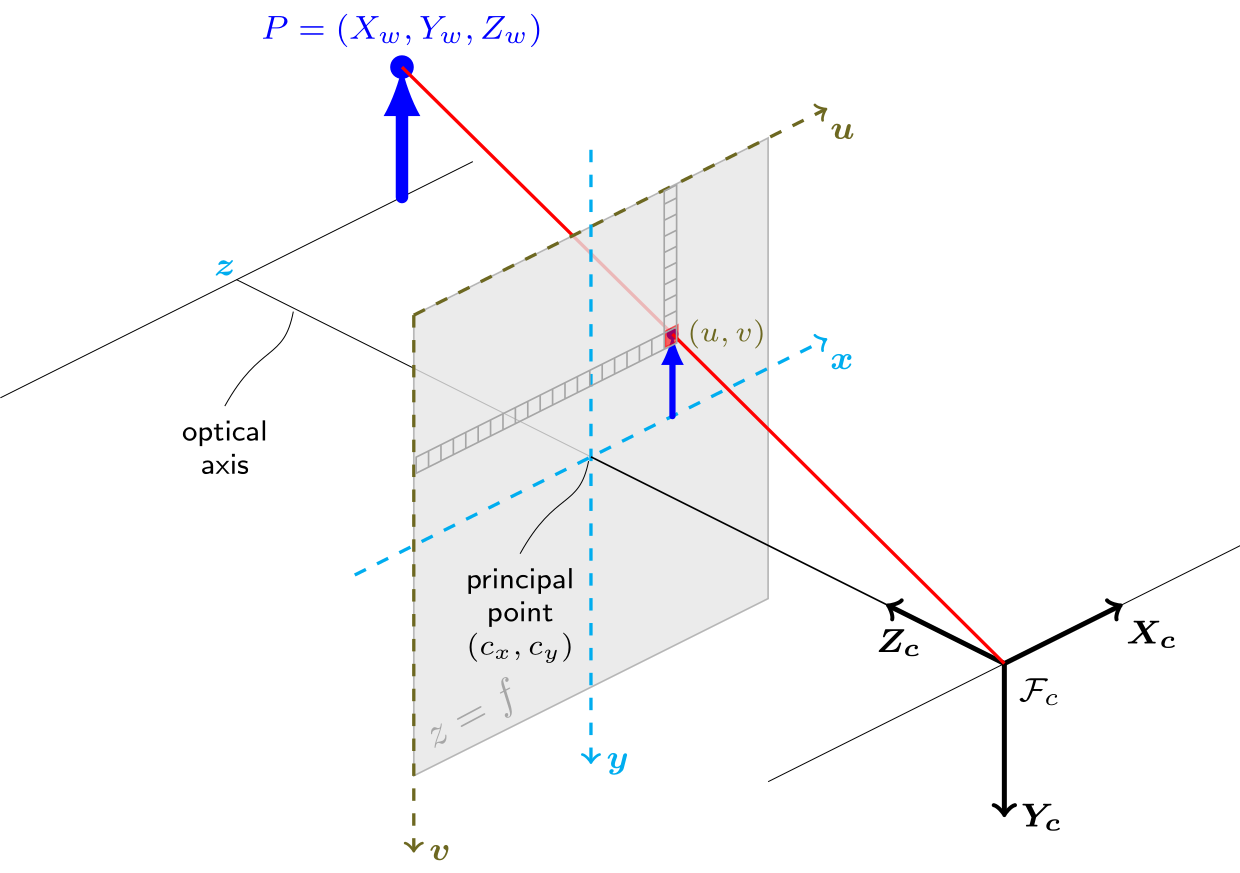
A camera sensor records the direction from which light reaches each pixel, not how far the light travelled. The pinhole model describes this. Every scene point sends one ray through a single point, the camera centre, and the place where that ray meets the image plane is where the point appears in the image. A real camera with a lens follows the same model closely, apart from lens distortion, which is covered in section 3.

In a physical pinhole camera the image forms behind the pinhole and is upside down. Computer vision uses a virtual image plane instead, placed at the same distance in front of the camera centre. The geometry is the same and the image is upright.

Figure 1. The pinhole camera model. A ray from the 3D point \(P\) passes through the camera centre, the origin of the camera frame \(\mathcal{F}_c\), and crosses the image plane \(z = f\) at pixel \((u, v)\). The optical axis meets the image plane at the principal point \((c_x, c_y)\), and pixel coordinates start at the top-left corner of the plane. The figure writes \(P\) in world coordinates \((X_w, Y_w, Z_w)\); in this post the world frame is the camera frame (see section 5), so these are the \((X, Y, Z)\) used in the text. Figure from the OpenCV documentation, calib3d module (Apache License 2.0).

2. Coordinate frames

Camera frame. The origin is the camera centre \(C\), also called the optical centre. The axes are:

\(X\) points right,
\(Y\) points down,
\(Z\) points forward along the optical axis, into the scene.

A point in front of the camera has \(Z > 0\), and \(Z\) is its depth.

Image frame. Pixel coordinates \((u, v)\) start at the top-left corner of the image, with \(u\) increasing to the right and \(v\) increasing downward. This matches how images are stored in memory.

Focal length. \(f\) is the distance from \(C\) to the image plane.

Principal point. \((c_x, c_y)\) is where the optical axis meets the image plane. It is usually close to the image centre, for example \((320, 240)\) in a 640 × 480 image.

3. The projection equations

Viewed from above, in the \(X\)–\(Z\) plane, the point \(P\) at horizontal offset \(X\) and depth \(Z\) and its image at offset \(x\) on the image plane form two similar right triangles that share the angle at \(C\):

\frac{x}{f} = \frac{X}{Z} \quad\Longrightarrow\quad x = f\,\frac{X}{Z}

The ratio uses the sides of the triangles, not the length of the ray. The image offset \(x\) is a physical length on the sensor, for example in millimetres, not a pixel coordinate.

To convert to pixels, divide by the pixel size and move the origin from the principal point to the top-left corner. With a lens of \(f = 2.5\) mm and 0.005 mm pixels, the focal length in pixels is

f_x = \frac{2.5\ \text{mm}}{0.005\ \text{mm per pixel}} = 500\ \text{px}

Doing the same for \(Y\) gives the projection equations:

u = f_x \, \frac{X}{Z} + c_x \qquad\qquad v = f_y \, \frac{Y}{Z} + c_y

\(f_x\) and \(f_y\) are the focal length in pixels along each axis. They are equal for square pixels.

Because \(X\) and \(Y\) are divided by \(Z\), a point twice as far from the camera lands half as far from the principal point. This is the source of perspective: distant objects appear smaller and closer to the image centre.

The same model can be written as one matrix, the intrinsic matrix:

K = \begin{bmatrix} f_x & 0 & c_x \\ 0 & f_y & c_y \\ 0 & 0 & 1 \end{bmatrix}

Multiplying \(K\) by a point gives

K \begin{bmatrix} X \\ Y \\ Z \end{bmatrix} = \begin{bmatrix} f_x X + c_x Z \\ f_y Y + c_y Z \\ Z \end{bmatrix}

and dividing the first two entries by the third, \(Z\), gives \(u\) and \(v\). Representing a pixel by a 3-vector and dividing by its last entry is called using homogeneous coordinates.

\(K\) is called intrinsic because it depends only on the camera's lens and sensor, not on where the camera is. The camera's position and orientation are described separately by the extrinsics, covered in section 5.

This form of \(K\) assumes no skew and no lens distortion. Real lenses bend straight lines, especially near the edges of wide-angle images. OpenCV models this with additional distortion coefficients, which are estimated together with \(K\) during camera calibration, usually from images of a checkerboard taken at different angles.

4. Worked example

Take a camera with \(f_x = f_y = 500\) px and principal point \((c_x, c_y) = (320, 240)\), and the point \(P = (1, 0.5, 5)\) m, which is 1 m to the right, 0.5 m below, and 5 m in front of the camera:

\begin{aligned} u &= 500 \cdot \frac{1}{5} + 320 = 100 + 320 = 420 \\[4pt] v &= 500 \cdot \frac{0.5}{5} + 240 = 50 + 240 = 290 \end{aligned}

The point appears at pixel (420, 290), to the right of and below the image centre. The matrix form gives the same result:

K P = \begin{bmatrix} 2100 \\ 1450 \\ 5 \end{bmatrix} \;\xrightarrow{\ \div\, 5\ }\; \begin{bmatrix} 420 \\ 290 \\ 1 \end{bmatrix}

Moving the same point to \(Z = 10\) m gives (370, 265), and \(Z = 20\) m gives (345, 252.5).

5. Implementation

NumPy

import numpy as np

def intrinsic_matrix(fx, fy, cx, cy):
    return np.array([[fx, 0.0, cx],
                     [0.0, fy, cy],
                     [0.0, 0.0, 1.0]])

def project(K, points_cam):
    """3D points in the camera frame (N x 3, metres) -> pixels (N x 2)."""
    P = np.atleast_2d(np.asarray(points_cam, dtype=float))
    if np.any(P[:, 2] <= 0):
        raise ValueError("all points must have Z > 0 (in front of the camera)")
    p_h = (K @ P.T).T              # homogeneous: (fx X + cx Z, fy Y + cy Z, Z)
    return p_h[:, :2] / p_h[:, 2:3]

K = intrinsic_matrix(500, 500, 320, 240)
print(project(K, [1.0, 0.5, 5.0]))   # [[420. 290.]]

Points with \(Z \le 0\) are behind the camera. The formula still returns a pixel for them, so they have to be filtered out before projecting.

OpenCV

cv2.projectPoints computes the same projection and also applies the camera pose and lens distortion:

import cv2
import numpy as np

points_3d = np.array([[1.0, 0.5, 5.0],
                      [2.0, 0.5, 5.0],
                      [1.0, 1.0, 5.0]])
K = np.array([[500, 0, 320],
              [0, 500, 240],
              [0, 0, 1]], dtype=np.float64)
rvec = np.zeros((3, 1))   # camera rotation (axis-angle): none
tvec = np.zeros((3, 1))   # camera translation: none
dist = np.zeros(5)        # lens distortion: none

pixels, _ = cv2.projectPoints(points_3d, rvec, tvec, K, dist)
print(pixels.reshape(-1, 2))
# [[420. 290.]
#  [520. 290.]
#  [420. 340.]]

The first row matches the worked example. Moving the point 1 m further right adds \(f_x \cdot \tfrac{1}{5} = 100\) px to \(u\), and moving it 0.5 m further down adds 50 px to \(v\).

rvec and tvec are the extrinsics. They move points from a world frame into the camera frame before projection:

P_{\text{camera}} = R \, P_{\text{world}} + t

Setting both to zero makes the world frame the same as the camera frame. Estimating \(R\) and \(t\) from images is the subject of Parts 4 to 6.

The repository's tests check that the NumPy function and cv2.projectPoints agree on a set of points.

6. From a pixel back to a ray

Different 3D points can project to the same pixel:

print(project(K, [[1.0, 0.5,  5.0],
                  [2.0, 1.0, 10.0],
                  [3.0, 1.5, 15.0]]))
# [[420. 290.]
#  [420. 290.]
#  [420. 290.]]

All three lie on the same ray through the camera centre, so the image cannot distinguish them.

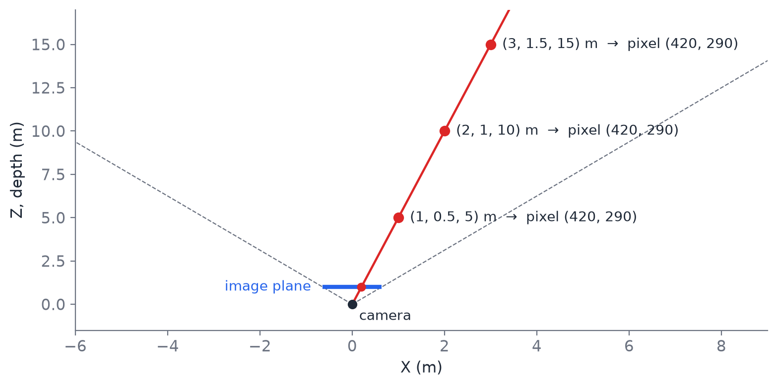
Three points on one ray hit the same pixel — Figure 2. Top-down view of three points at depths of 5, 10, and 15 m on one ray through the camera. All three project to pixel (420, 290).

Inverting the projection therefore gives a ray, not a point. For a pixel \((u, v)\), each depth \(Z\) selects one point on that ray:

P = Z \, K^{-1} \begin{bmatrix} u \\ v \\ 1 \end{bmatrix}

ray = np.linalg.inv(K) @ np.array([420, 290, 1.0])
print(ray)          # [0.2 0.1 1. ]   ray direction, scaled so Z = 1
print(5.0 * ray)    # [1.  0.5 5. ]   the original point, given Z = 5

Recovering the 3D point needs its depth, which a single image does not provide. VO systems obtain it in different ways:

Stereo cameras observe the same point from two cameras a known distance apart and compute its depth from the difference in position between the two images (Part 2).
Monocular VO recovers the direction of camera motion but not its magnitude, because scaling the scene and the motion together leaves every pixel unchanged (Part 6).
Additional sensors, such as an IMU, wheel encoders, or a depth sensor, provide metric scale. In my work on monocular SLAM for assistive smart glasses, a small time-of-flight sensor serves this purpose.

7. Where this is used in the series

Part	Topic	Use of the projection model
2	Stereo depth	Two projections of the same point from cameras a known distance apart determine its depth.
3	Feature matching	Finds the same physical point in two images, which are two projections of one 3D point.
4	Motion from 3D points (Kabsch, RANSAC)	Back-projects matched pixels with known depth into 3D points, then finds the rotation and translation that align them between frames.
5	PnP and reprojection error	Finds the camera pose under which known 3D points project onto the observed pixels. The remaining pixel distance, the reprojection error, is the main error measure in VO and SLAM.
6	Monocular VO	Inverts the projection across two frames, up to an unknown scale.
7	End-to-end pipeline	Runs Parts 2 to 6 on a real image sequence and evaluates the resulting trajectory.
8	Pose-graph optimization	Refines camera poses so the trajectory is consistent with the relative motions estimated from images.

The series follows the classic feature-based pipeline. Many current systems instead track features with optical flow, align pixel intensities directly (direct methods such as DSO), or learn correspondences with a network (DROID-SLAM, DPVO). These approaches differ in how they relate pixels across frames, but all of them use the same projection model.

Part 2 adds a second camera at a known distance \(B\) from the first. The horizontal shift of a point between the two images, its disparity \(d\), gives its depth through \(Z = f_x B / d\).

The code for this post and its tests are in the repository under part01_camera_geometry/:

pip install -r requirements.txt
python part01_camera_geometry/demo.py    # draws Figure 2
pytest tests                             # checks the projection, including against OpenCV

References

Camera model and projection (sections 1 to 4)

R. Hartley and A. Zisserman, Multiple View Geometry in Computer Vision, 2nd ed. Cambridge University Press, 2004. Chapter 6, "Camera Models". Book page
R. Szeliski, Computer Vision: Algorithms and Applications, 2nd ed. Springer, 2022. Chapter 2, "Image formation". Free online

Calibration and lens distortion (section 3)

Z. Zhang, "A flexible new technique for camera calibration," IEEE Transactions on Pattern Analysis and Machine Intelligence, 22(11):1330–1334, 2000. doi:10.1109/34.888718
OpenCV, "Camera Calibration" tutorial. docs.opencv.org

Code (sections 5 and 6)

OpenCV, "Camera Calibration and 3D Reconstruction" (calib3d module): the pinhole model, the distortion model, and cv2.projectPoints. docs.opencv.org

Visual odometry

D. Nistér, O. Naroditsky, and J. Bergen, "Visual odometry," in Proc. IEEE Conference on Computer Vision and Pattern Recognition (CVPR), 2004, pp. 652–659. doi:10.1109/CVPR.2004.1315094
D. Scaramuzza and F. Fraundorfer, "Visual Odometry [Tutorial]," IEEE Robotics & Automation Magazine, 18(4):80–92, 2011. doi:10.1109/MRA.2011.943233
F. Fraundorfer and D. Scaramuzza, "Visual Odometry: Part II: Matching, Robustness, Optimization, and Applications," IEEE Robotics & Automation Magazine, 19(2):78–90, 2012. doi:10.1109/MRA.2012.2182810

Methods named in section 7

J. Engel, V. Koltun, and D. Cremers, "Direct Sparse Odometry," IEEE Transactions on Pattern Analysis and Machine Intelligence, 40(3):611–625, 2018. doi:10.1109/TPAMI.2017.2658577
Z. Teed and J. Deng, "DROID-SLAM: Deep Visual SLAM for Monocular, Stereo, and RGB-D Cameras," NeurIPS, 2021. arXiv:2108.10869
Z. Teed, L. Lipson, and J. Deng, "Deep Patch Visual Odometry," NeurIPS, 2023. arXiv:2208.04726